Using Google Spreadsheets (or Excel) to Chart Your Success Through Life
This post originally appeared in my other blog, Living For Improvement. However, given the technical nature of the lifehack at hand, I decided to cross-post it here. Enjoy!
For years now, I’ve been using a system called Key Lifestyle Indicators (KLIs) that I modeled after the idea of Key Performance Indicators in business.
My KLI definitions have changed over the years; here’s my current set-up:
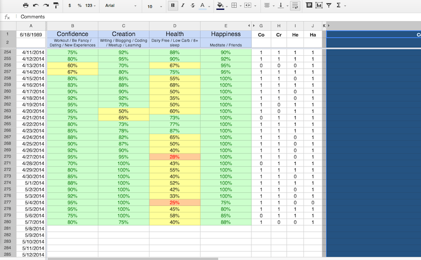
This system works very well for me, consistently reminding me where I’m slacking and where I’m succeeding. The best part: it requires less than 10 seconds per day to enter the necessary information (nowadays it’s simply 1s and 0s transformed into a moving average).
It wasn’t until this past week that I found a way to leverage this tracked data in a new, interesting way. The inspiration came from reading Wait But Why’s post on what your life looks like plotted out into weeks (hint: You have less than 4,500 weeks in your life to spend – how have you been using them?).
I loved the idea of a meaningful reminder of the limited number of weeks we have on this planet. Thankfully, Wait But Why offers some sweet calendars that allow you to track how you’re living out your weeks – either with hand-scribbled notes or via color coding.
I’ll probably pick up one of these awesome calendars some time in the near future, but I wondered if I could use my years of KLI data to graphically represent this without needing to create yet another place to track my progress through life.
This post describes how I took my KLI data and created a Wait-But-Why-styled life calendar that lives in Google Spreadsheets (or Excel, if that’s your thing). If you track similar data in a spreadsheet, this article should help you in creating a similar set-up (read Wait But Why’s post for a deeper understanding of why a life calendar is awesome).
Step 1: Prototype the end result
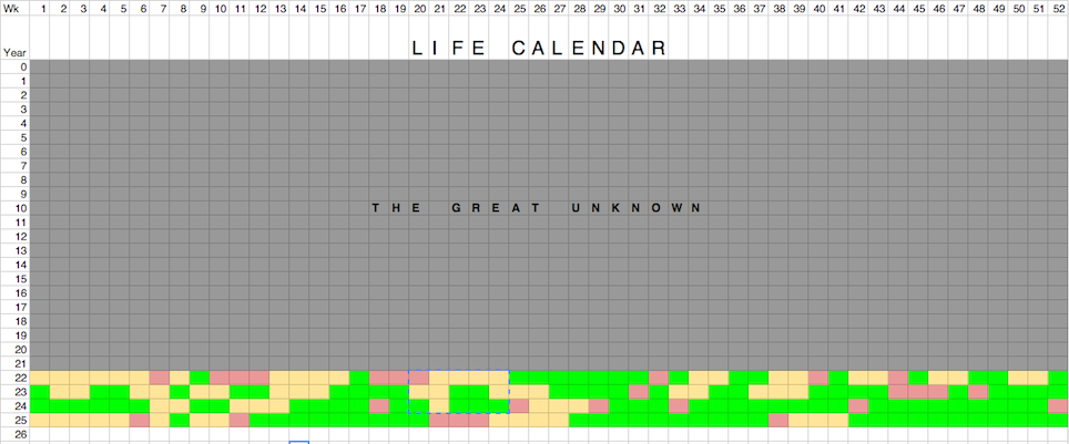
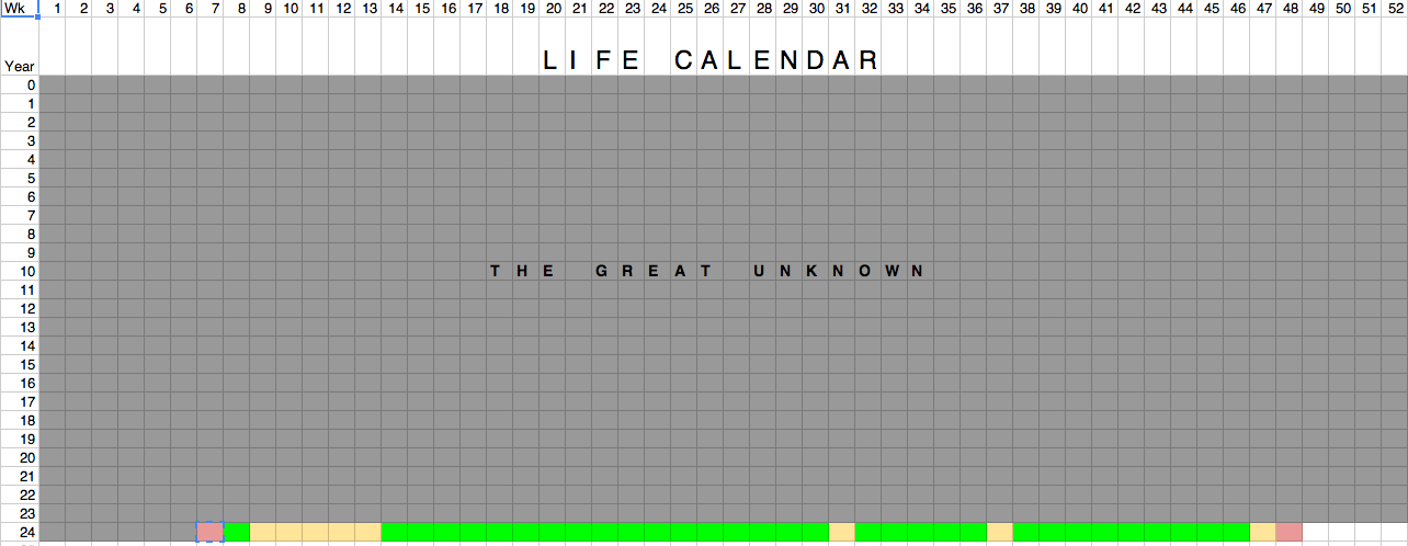
Here’s what I wanted my life calendar to look like when all was said and done:

Note how I keep untracked weeks in gray, but everything else is colored yellow, green, or red depending on how my KLIs looked that week. The goal was to have this automatically calculated for me, as manually-inputted tracking can get quite annoying. But in order for this to become automated, I needed to pull together all of the necessary data, which brings me to step 2…
Step 2: Survey the current datascape
The calendar prototype looked good, but the data I needed was siloed in different cells. In other words, because none of the data was rolled up by day or week, some intermediary data compilation was required before the calendar could pull what it needed.
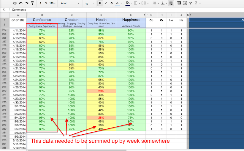
Step 3: Compile the calendar data
After surveying my data, I realized I needed to compile my data in two ways to transition to the life calendar:
- Daily score sums…
- …rolled up into weekly score sums
I ended up adding two additional columns into my KLI sheet (which I now keep hidden) to accomplish step 1. See below:
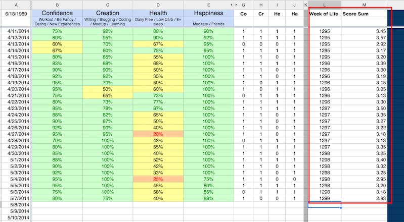
I calculated the week of my life (Column L) using this formula: =ROUNDDOWN((CURRENT_DATE - DATE_I_WAS_BORN +1)/7). The +1 in that formula ensures that the calculation includes today’s date when rounding down to the current week.
From there, I summed up each day’s scores using the sum of columns B, C, D, and E. For example, for the day on row 50, the M50 cell contained =B50+C50+D50+E50.
For step 2, I used a pivot table to keep an up-to-date weekly summary of my scores:
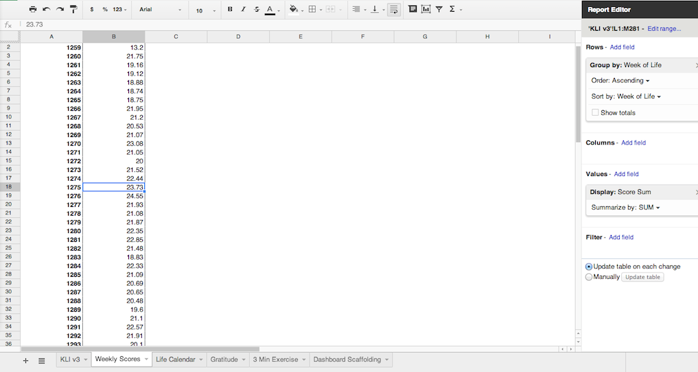
It rolls up all of the scores by week using the two new columns I showed in the previous screenshot. With my daily scores summed and rolled up by week, it was time to link this data to my calendar prototype.
Step 4: Bring the calendar to life
This step was the most time intensive, so I broke into three main tasks:
A. Link the data points to the calendar
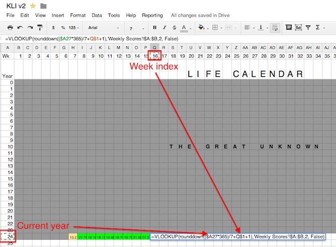
This task involved a VLOOKUP formula to pull the right score based on week. To pull from the right place in the pivot table, I simply needed to calculate the current week and then do the VLOOKUP. It’s a little heavy to look at, but it ended up looking like this: =VLOOKUP(rounddown((CURRENT_YEAR*365)/7 + WEEK_INDEX+1),'Weekly Scores'!$A:$B,2, False)

Here’s a broader view with cell highlighting. Notice how it uses the Week Index and the current year to calculate the correct week of my life, and then runs the VLOOKUP based on that value:
B. Handle errors
Although the VLOOKUP worked quite well, there were two errors I had to account for:
-
The formula returns an error for future weeks that haven’t been calculated yet.
-
A particular oddity with Google Spreadsheets was causing the VLOOKUP to lock the formula in place and make it uneditable (turns out this is a Google Spreadsheets bug when doing a VLOOKUP on pivot tables – hopefully this gets fixed soon).
To solve the first issue, it was rather easy. I wrapped the VLOOKUP in an IFERROR like so:
=IFERROR(VLOOKUP_GOES_HERE, "")
This made sure that the formula returned an empty string for future weeks, keeping the calendar clean and error-free.
To solve the second issue, I used a trick I found on Stack Exchange. The trick involves arbitrarily adding a +0 to your VLOOKUP calculation. This won’t skew the calculation, obviously, and for some reason keeps the cell formula editable.
Here’s what the VLOOKUP looked like with the +0 added in:
VLOOKUP(rounddown((CURRENT_YEAR*365)/7 + WEEK_INDEX+1),'Weekly Scores'!$A:$B,2, False)+0
Problem solved!
With both errors handled, the final formula looked like this:
=IFERROR(VLOOKUP(rounddown((CURRENT_YEAR*365)/7 + WEEK_INDEX+1),'Weekly Scores'!$A:$B,2, False)+0, "")
C. Set up conditional formatting rules
With the hard part out of the way, all I needed to do was make the cells color coded based on my score that week.
In my KLI system, the ideal day would earn me 4 points. Therefore, my ideal week would yield 28 points. With that in mind, here’s how I defined and color-coded great, ok, and bad weeks.
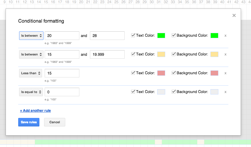
As you can see, 20 points or above is a good week, 15-20 points is a so-so week, and anything less is a red flag. Also notice how I alter the text color as well to hide the number calculation that lives in the cell.
Step 5: Celebrate!
At this point, I took a step back and appreciated my sexy, new life calendar, auto-calculated based on the KLI system I’ve trusted for years.
Tim Urban, if you’re reading this post, I just want to say thank you for the inspiration. I follow your blog religiously, and this obviously could not have come about without your wisdom. Cheers mate.
Now, off to appreciate the precious weeks I have left.